Comprehensive Guide to Optical Transceivers: 1G to 800G Architecture, Components, and Applications
Introduction
In modern data centers and telecommunications networks, optical transceivers serve as the critical bridge between electrical and optical domains. A common question arises: “Are switches optical switching devices?” The answer is nuanced—optical transceivers combined with switches form a complete optical switching system. Today’s data center Ethernet switches are essentially optical communication devices, as the entire system operates on optical transmission principles.
1. Physical Architecture and Interface Design
1.1 Understanding the Optoelectronic Conversion Role
Critical Distinction: An optical transceiver is an optoelectronic converter, not a purely optical device. This is a fundamental concept that must be emphasized. One side connects electrically to switches or network cards, while the other side connects optically to fiber cables. The device performs bidirectional conversion between these two domains.
On the transmit path, it converts high-speed electrical signals from switches or network interface cards into modulated optical signals suitable for fiber transmission. Conversely, on the receive path, it reconverts incoming optical signals back into electrical format for processing by host devices.
1.2 External Structure and Critical Physical Components
Key Physical Elements
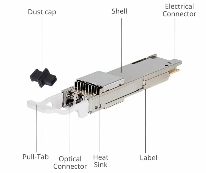
Modern optical transceivers incorporate several essential external components:
- Electrical Connector: Interfaces with host equipment (switches, routers, NICs) on one side
- Optical Connector: Connects to fiber optic cables, available in various configurations (LC, MPO/MTP, MXC) depending on application requirements
- Heat Sink: A critical component, especially for high-speed modules. Modern 400G and 800G transceivers consume 10W or more, making thermal management essential. The heat sink is mandatory for these power levels and may even include a dedicated cooling module—essentially a “mini air conditioner” that itself consumes power. This level of sophistication demonstrates that optical transceivers are precision instruments.
- Pull-Tab with Color Coding: Different speeds and transmission distances use different color pull-tabs, providing visual identification in data centers:
- Beige/Tan: 850nm wavelength (50-100m multimode applications)
- Yellow: DR applications (500m)
- Green: FR applications (2km)
- Blue: 1310nm wavelength
- White: 1550nm wavelength (long-haul applications)
- Protective Shell and Dust Cap: Shields internal components and optical interfaces from environmental contamination
1.3 Evolution of Form Factors
The industry has witnessed continuous evolution in transceiver form factors, driven by demands for higher bandwidth density and improved power efficiency. It’s important to note that the physical size progression doesn’t perfectly match the diagrams—SFP is actually the smallest, QSFP is medium-sized, and OSFP is the largest, reflecting the evolution from lower to higher conversion capabilities.
SFP Family (Small Form-factor Pluggable)
- Dimensions: 13.4 × 8.5 × 56.5 mm
- Bandwidth progression:
- SFP (1G) → SFP+ (10G) → SFP28 (25G)
- SFP112 (100G): New upgrade supporting higher-speed optical channels
- SFP-DD (200G): Essentially two SFP modules combined
- Power envelope: <1W to <3W depending on variant
- Primary use: Lower-density applications, backward compatibility requirements
QSFP Family (Quad Small Form-factor Pluggable)
- Critical Terminology Note: “QSFP” is not a fixed designation. Originally referring to QSFP28 (4×28G lanes), the term has evolved:
- QSFP28: 4×28 Gbps = 100G
- QSFP56: 4×56 Gbps = 200G
- QSFP112: 4×112 Gbps = 400G
- QSFP112-DD: 8×112 Gbps = 800G
- Dimensions: 18.35 × 8.5 × 72.0 mm (standard) to 89.0 mm (DD variants)
- Power envelope: <1W to 15W depending on variant
- Primary use: High-density data center deployments, mainstream applications
OSFP Family (Octal Small Form Factor Pluggable)
- Dimensions: 22.58 × 13 × 100.4 mm (standard) to 124.8 mm (XD variant)
- Latest developments:
- OSFP-1.6T: 1.6 Tbps capability
- OSFP-XD: 3.2 Tbps capability
- Power envelope: <15W to >20W
- Primary use: Next-generation high-bandwidth applications, AI/ML infrastructure
Comparison of Transceivers Form Factors
| Standard | Max. Speed | Channels | Bandwidth | Power Consumption | Size (mm) |
| SFP | 1 Gbps | 1 | 1 Gbps | < 1 W | 13.4 × 8.5 × 56.5 |
| SFP+ | 10 Gbps | 1 | 10 Gbps | < 1 W | 13.4 × 8.5 × 56.5 |
| SFP28 | 28 Gbps | 1 | 25 Gbps | < 1.5 W | 13.4 × 8.5 × 56.5 |
| SFP112 | 112Gbps | 1 | 100Gbps | < 2 W | 13.4 × 8.5 × 56.5 |
| SFP-DD | 112Gbps x 2 | 2 | 200Gbps | < 3 W | 13.4 × 8.5 × 56.5 |
| QSFP | 1 Gbps × 4 | 4 | 4 Gbps | < 1 W | 18.35 × 8.5 × 72.0 |
| QSFP+ | 10 Gbps × 4 | 4 | 40 Gbps | < 2 W | 18.35 × 8.5 × 72.0 |
| QSFP28 | 28 Gbps × 4 | 4 | 100 Gbps | < 3.5 W | 18.35 × 8.5 × 72.0 |
| QSFP56 | 56 Gbps × 4 | 4 | 200 Gbps | < 5W | 18.35 × 8.5 × 72.0 |
| QSFP56-DD | 56 Gbps × 8 | 8 | 400 Gbps | 8-12 W | 18.35 × 8.5 × 89.0 |
| QSFP112 | 112 Gbps × 4 | 4 | 400 Gbps | 6-8 W | 18.35 × 8.5 × 89.0 |
| QSFP112-DD | 112 Gbps × 8 | 8 | 800 Gbps | 10-15 W | 18.35 × 8.5 × 89.0 |
| OSFP | 56 Gbps × 8 | 8 | 400 Gbps | < 15 W | 22.58 × 13 × 100.4 |
| OSFP112 | 112 Gbps × 8 | 8 | 800 Gbps | 15-20 W | 22.58 × 13 × 100.4 |
| OSFP-1.6T | 224 Gbps × 8 | 8 | 1.6 Tbps | >20W | 22.58 × 13 × 100.4 |
| OSFP-XD | 224 Gbps × 16 | 16 | 3.2Tbps | 22.58 × 13 × 124.8 |
1.4 Multi-Channel Parallel Transmission Architecture
Why Parallel Transmission?
Due to physical limitations of lasers, detectors, and fiber capacity, single-lane transmission rates have reached practical limits around 200 Gbps (previous generation at 100 Gbps). To achieve 800G speeds, we combine eight 100G channels, which requires multi-channel parallel transmission in optical fiber communication.
Spatial Division Multiplexing (SDM) – Multi-Fiber Transmission
SDM employs multiple independent fiber paths for short-distance applications:
- QSFP-DD SR8: Utilizes 8 fiber pairs (16 fibers total) via MPO-16 connector
- QSFP-DD 2×SR4: Employs dual MPO-12 connectors—two groups of 4 lanes each
Key Insight: What appears as a single optical cable actually contains multiple individual fibers inside. For example, a common QSFP-DD SR8 uses 8 fiber pairs (8 transmit, 8 receive) totaling 16 fibers through an MPO-16 connector.
Advantages: Straightforward implementation, mature technology, excellent channel isolation.
Limitations: High fiber count requirements, primarily for short-distance use.
Wavelength Division Multiplexing (WDM) – Multi-Wavelength Transmission
For long-distance transmission, instead of multiple fiber pairs, WDM uses a single fiber pair (one transmit, one receive) but distinguishes channels through different wavelengths:
- Example: 400G FR4: Uses four wavelengths, each carrying one signal channel, achieving multiplexing on a single fiber
- SWDM (Short Wavelength Division Multiplexing): 850-953nm range on OM5 multimode fiber, 4 wavelengths, 30-150m reach
- CWDM (Coarse WDM): 1270-1610nm range on single-mode fiber, 8-18 wavelengths, 10-40km reach
- LWDM (LAN WDM): 1260-1360nm range optimized for data center applications, 12 wavelengths
- DWDM (Dense WDM): 1530-1625nm range (C+L bands), 40-80+ wavelengths, 80km to thousands of kilometers
Advantages: Minimal fiber infrastructure, scalable capacity, efficient for long-haul.
Limitations: Higher component complexity, wavelength stability requirements, and increased cost.
Bidirectional (BiDi) Technology
A clever multiplexing approach where:
- Two fibers exist, but one fiber is used only for transmission, the other only for reception
- On one side of the transceiver: one transmit, one receive
- On the opposite side: the roles reverse (receive becomes transmit)
- Important: BiDi modules are sold in pairs and must be used together
Application: Specialized BiDi optical modules available for specific use cases encountered in projects
1.5 Optical Connector Technologies
Critical Compatibility Principle: Whether two optical modules can interconnect depends primarily on their optical signal compatibility, NOT the electrical connector type. Even if one module uses OSFP and another uses QSFP electrical connectors, they can interconnect if their optical signals are compatible.
Optical Connector vs. Optical Signal: The optical connector interface differs from the optical signal itself. Breakout cables can convert between connector types (e.g., MPO to LC) while maintaining signal compatibility if the internal optical signals match (e.g., all 112G lanes, or all 56G lanes, or all 28G lanes).
MPO/MTP Multi-Fiber Connectors
MPO (Multi-fiber Push-On) and its enhanced variant MTP (Multi-fiber Termination Push-on) are compatible protocols—MTP is an upgraded version created by a specific company but widely accepted. These terms are often used interchangeably.
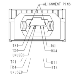
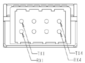
MPO-12
12 fibers – 4 unused
1 cable
TX/RX or TR model
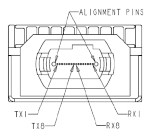
MPO-16
16 fibers
1 cable
TX/RX model
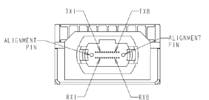
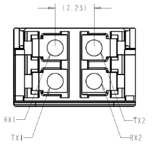
MPO-12 Two Row
24 fibers – 8 unused
1 cable
TX/RX model
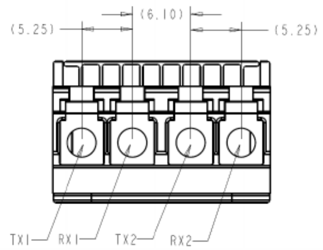
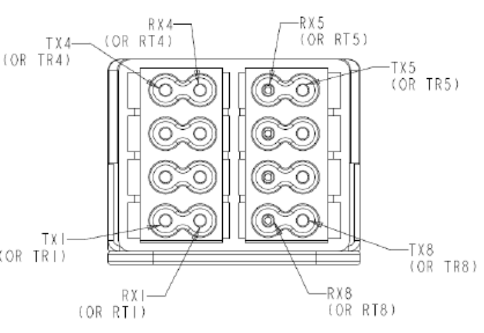
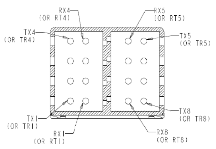
Dual MPO-12
24 fibers – 8 unused
2 cables
TX/RX model
Configurations:
- MPO-12: 12 fibers (typically 8 active, 4 unused), single cable, commonly paired with 4-channel optical signals
- MPO-16: 16 active fibers, single cable, optimized for 8-lane transceivers, supports 8-channel optical signal transmission
- MPO-12 Two Row: 24 fibers (16 active) in stacked configuration, single cable (rarely used)
- Dual MPO-12: 24 fibers (16 active) across 2 cables—Very common configuration
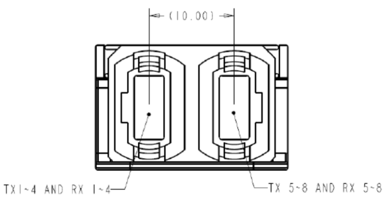
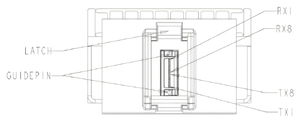
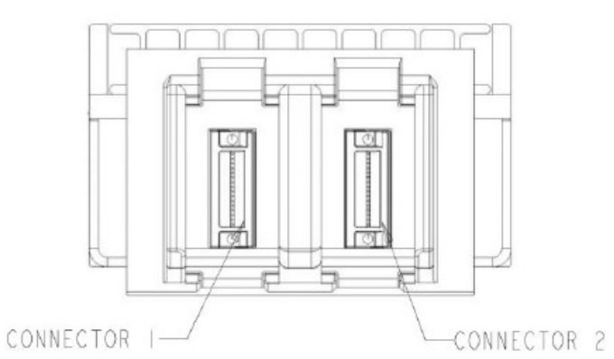
- Critical 800G Implementation Detail: The vast majority of current 800G optical modules use this dual MPO-12 format
- Architectural Significance: This means 800G modules are essentially two physically separate 400G modules integrated into a single OSFP form factor
- The two optical ports (two MPO-12 connectors) are physically isolated from each other
- Project Implication: When customers ask “Why don’t you provide 400G interfaces?” explain that one 800G optical module equals two 400G modules with physical isolation
Technical Characteristics:
- Alignment precision: ±0.75 μm (MTP) vs ±1.5 μm (standard MPO)
- Typical insertion loss: <0.35 dB (MTP), <0.5 dB (MPO)
- Return loss: >20 dB for PC, >60 dB for APC
- Fiber compatibility: Single-mode and multimode variants available
- Primary Application: Short-distance transmission (mainly <100m, though some extend to 2km)
MXC Next-Generation Connector
MXC (Multi-Fiber eXpandable Connector) represents cutting-edge technology for future higher-speed requirements:
Key Features:
- Higher Fiber Count: Dual MXC supports 32 fibers for 16 channels
- Next-Generation Ready:
- 16 channels × 100G = 1.6T
- 16 channels × 200G = 3.2T
- Primary applications: Co-Packaged Optics (CPO), silicon photonics integration, AI/HPC clusters designed for next-generation requirements
MXC
16 fibers
1 cable
TX/RX model
Dual MXC
32 fibers
2 cables
TX/RX model
LC Duplex and Variants
LC (Lucent Connector), invented by Lucent Technologies, remains predominant for lower-density and longer-reach applications:
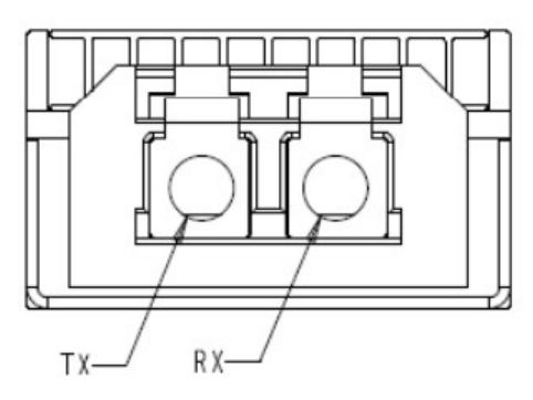
Duplex LC
2 fibers
1 cable
TX/RX model
Dual Mini-LC
4 fibers
2 cables
TX/RX model
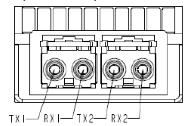
Dual Duplex LC
2 x 2 fibers
2 cables
TX/RX model
Dual CS LC
4 fibers
2 cables
TX/RX model
Standard Configurations:
- Duplex LC: 2 fibers (TX/RX pair), 8.1 × 2.5 mm footprint
- Terminology Note: “Duplex LC” is somewhat redundant since LC is inherently duplex (one transmit, one receive)
- However, the term is still commonly used
- Dual Duplex LC: 4 fibers across 2 duplex LC connections
- CRITICAL DISTINCTION: “Dual Duplex LC” ≠ “Duplex LC”
- “Duplex” = duplex/bidirectional nature
- “Dual” = two sets/pair of connections
- Common in: FR4/LR4 applications requiring 4-wavelength WDM
- Warning: Confusing these terms can lead to incorrect module orders and costly returns
- Dual Mini-LC / Dual CS LC: Compact variants offering 2-3× density improvement
Technical Characteristics:
- Insertion loss: <0.3 dB typical
- Return loss: >50 dB (APC), >35 dB (PC)
- Connector endface: 1.25mm ceramic ferrule
- Usage Pattern: Very common in low-speed modules; even short-distance low-speed applications use LC
- Application Range: Suitable for both short and long distances, especially prevalent in lower-speed modules
Emerging High-Density Connectors
- MDC (Miniature Duplex Connector): 2× density vs. LC, 4.5 × 1.6 mm, optimized for 5G transport networks
- SN (Senko Advanced Components): 3× density vs. LC, 2.0 × 6.0 mm, designed for hyperscale data centers
Future Outlook: These will become more relevant when 1.6T and 3.2T modules become mainstream
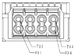
Quad MDC
8 fibers
4 cables
TX/RX or TR model
Quad SN
8 fibers
4 cables
TX/RX or TR model
8 x MDC
2 x 8 fibers
8 cables
TX/RX
8 x SN
2 x 8 fibers
8 cables
TX/RX model
Comparison of Optical Connectors
| Fiber Connector | Fiber# | Size (W x H, mm) |
| MPO-12 | 12 | 12.4 x 6.4 |
| MPO-16 | 16 | 12.4 x 6.4 |
| Dual MPO-12 | 24 | 12.8 x 12.4 |
| MPO-12 Two Row | 24 | 12.4 x 9.5 |
| SC (Subscriber Connector) | 1 | 8.8 x 8.5 |
| LC (Lucent Connector) | 1 | 5.5 x 2.5 |
| Duplex LC | 2 | 8.1 x 2.5 |
| Dual Duplex LC | 4 | 13.1 x 6.6 |
| Dual Mini LC | 2 | 11.7 x 2.5 |
| Dual CS LC | 2 | 7.2 x 2.0 |
| MXC (Multi-Fiber eXpandable) | 16 | 21.2 x 10.2 |
| Dual MXC | 32 | 20.4 x 21.2 |
| MDC(Miniature Duplex Connector) | 2 | 4.5 x 1.6 |
| SN | 2 | 2.0 x 6.0 |
1.6 Transmission Distance Classifications
Data Center Common Distance Abbreviations:
| Category | Distance | Fiber Type | Wavelength | Typical Application |
| VR (Very Short Range) | 50m | OM3/OM4 MMF | 850nm | GPU interconnect, intra-rack, server-to-ToR |
| SR (Short Range) | 100m | OM3/OM4 MMF | 850nm | Inter-rack, short ToR-to-Spine |
| DR (Data Center Reach) | 500m | SMF | 1310nm | Intra-building, floor-to-floor |
| XDR (eXtended DR) | 2km | SMF | 1310nm | Campus interconnect, extended DC |
| FR (Front Range) | 2km | SMF | 1310nm | POD-to-POD, metro access |
| LR (Long Range) | 10km | SMF | 1310nm | Inter-DC, metro aggregation |
| ER (Extended Range) | 40km | SMF | 1550nm | DCI, metro core |
| ZR (Zonal Reach) | 80km | SMF | 1550nm | Regional DCI, metro edge |
| ZR+ | 120km+ | SMF | 1550nm | Long-haul DCI, inter-city |
VR vs. SR: Important Distinction
Why VR Emerged: In data centers, especially for GPU interconnects, 50 meters is often sufficient. By limiting distance to 50m, manufacturers can achieve:
- Lower cost compared to SR modules
- Better optical transmission characteristics
- Improved performance metrics
Industry Context: NVIDIA pioneered this standard and calls it “SR” in their documentation, but the industry generally uses “VR” to distinguish it from traditional 100m SR modules.
Key Differences:
- VR: 50m, slightly cheaper, optimized for short GPU interconnect scenarios
- SR: 100m, slightly more expensive, broader compatibility
Customer Value: Both help reduce total data center costs by matching capability to actual requirements
XDR Technology Note
XDR Characteristics:
- Uses single-mode fiber or single-wavelength approach
- Multi-channel spatial division extending to 2km
- Competitive relationship with FR (FR currently more common)
- Both target the 2km distance category but use different technical approaches
1.7 Multimode Fiber Specifications
Commonly Used: OM3 and OM4 are the mainstream choices for 50m-100m applications
OM5 Position: Despite longer transmission distances, OM5 is somewhat awkward:
- Higher cost than OM3/OM4
- Limited adoption because most optical modules are designed for 50-100m ranges
- The extra distance capability often goes unused, making the premium less justified
| Grade | Core Diameter | Bandwidth | Wavelength | Max Distance (800G) | Common Use |
| OM1 | 62.5 μm | 200 MHz·km | 850nm | Legacy only | Obsolete |
| OM2 | 50 μm | 500 MHz·km | 850nm | Legacy only | Obsolete |
| OM3 | 50 μm | 2000 MHz·km | 850nm | 50m | Very Common |
| OM4 | 50 μm | 4700 MHz·km | 850nm | 100m | Very Common |
| OM5 | 50 μm | 28000 MHz·km | 850-953nm | 150m (SWDM capable) | Less common, expensive |
1.8 Wavelength Division Multiplexing Technologies
| Technology | Fiber Type | Wavelength Range | Channel Count | Distance | Typical Application |
| SWDM | MMF (OM5) | 850-953nm | 4 | 30-150m | Data center short-reach, 100G/400G/800G |
| CWDM | SMF | 1270-1610nm | 8-18 | 10-40km (up to 80km) | Medium-distance, DCI |
| LWDM | SMF | 1260-1360nm | 12 | 10-40km | Medium-distance, DCI |
| DWDM | SMF | C-band: 1530-1565nm L-band: 1565-1625nm | 40-80+ | 80km – thousands of km | Long-haul transmission |
Data Center Usage: SWDM and CWDM are most commonly encountered in data center environments
1.9 Thermal Management Solutions
Critical Importance: From 400G onwards, especially with 800G modules, thermal management has become a serious challenge.
OSFP Heat Sinks
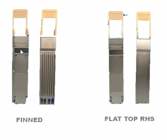
Fin-Top Configuration (13mm height):
- High-power design: For modules >15W
- Finned surface: Maximized heat dissipation area
- Primary use: Switch-side optical modules
- Example: CX864E switch uses Fin-Top configuration
Flat-Top/RHS Configuration (8.5mm height):
- Standard power design: For modules <15W
- Lower profile: Space-constrained applications
- Primary use: NIC-side/Host-side optical modules
- Reason for host-side use:
- NICs have sufficient space
- Better cooling conditions on host side
- NIC card slots often include integrated heat sinks
- NVIDIA BlueField DPUs and ConnectX NICs use RHS format
Critical Procurement Note:
- Switch-side (e.g., CX864E): Order Fin-Top format
- NIC-side (e.g., NVIDIA ConnectX/BlueField): Order RHS/Flat-Top format
- Mixing these up requires module replacement—costly mistake!
QSFP112/QSFP112-DD Heat Sinks

Type 1/2 (8.5mm height):
- Standard thermal performance
- Mainstream 400G/800G modules
- Not as prominent as OSFP heat sinks
Type 2A/2B (8.5mm height):
- Enhanced thermal conductivity
- High-power variants
- All types maintain 8.5mm height
Comparison to OSFP:
- Less dramatic heat sink design than OSFP
- Smaller additional heat dissipation area beyond main body
- Thermal performance: Lower than OSFP (explains why the CX864E 800G switch uses the OSFP format)
- Suitable for: Host systems or liquid-cooled switch systems with superior ambient cooling
1.10 Color-Coded Pull-Tabs
OSFP Official Standards: Well-defined color coding system
QSFP Official Standards: Simpler definitions:
- Beige: 850nm
- Blue: 1310nm
- White: 1550nm
Industry Practice: QSFP implementations typically follow OSFP color standards for consistency
Common Color Scheme (Both OSFP and QSFP in practice):
- Beige/Tan: 50m and 100m (VR/SR)
- Yellow: 500m (DR)
- Green: 2km (FR)
- Blue: Longer distances (LR and beyond)
Additional Conventions:
- DAC (Direct Attach Copper): Typically black (copper cable)
- AOC (Active Optical Cable): Often gray
- These are the most commonly encountered colors
Practical Value: At-a-glance identification in data center environments
2. Internal Architecture and Critical Components
2.1 Core Components: The Three Pillars
Three Most Critical Components:
- Laser (Transmitter): Optical transmission device
- Detector (Receiver): Optical reception device
- DSP (Digital Signal Processor): Electronic processing module
Logical Signal Path:
Transmit Path:
Electrical Signal → DSP Processing → Driver → Laser (TOSA) → Filtered Light → Optical OutputReceive Path:
Optical Input → Detector (ROSA) → TIA (Current to Voltage) → DSP Processing → Electrical SignalComponent Functions:
- DSP: Performs signal conditioning before transmission
- Driver: Electronic component that drives the laser to emit light at different wavelengths, modulating it into optical signals
- Optical Filter: Filters specific wavelengths before transmission
- Detector: Receives optical data, outputs weak current signal
- TIA (Transimpedance Amplifier): Converts weak photodiode current to voltage and amplifies it for DSP processing
2.2 Power Consumption Analysis: The Surprising Truth
Question: Which components consume the most power?
Answer (May Surprise You): DSP is the biggest power consumer, NOT the optical components
Power Distribution (7nm DSP example):
- DSP: 59% of total power (7nm process)
- 5nm DSP: Even higher at 65%
- Laser: ~10% (needs power to emit light)
- TIA: ~10% (needs power to amplify weak detector signals)
- TEC (Thermoelectric Cooler): Significant portion
- Functions as module’s “air conditioner”
- Consumes electricity to provide cooling
- Keeps module within acceptable temperature range
Key Insight: This sophisticated power architecture demonstrates why optical transceivers are precision instruments deserving of their premium pricing.
2.3 TOSA (Transmitter Optical Sub-Assembly)
TOSA integrates the laser and peripheral components into a unified transmit-side optical sub-module responsible for electrical-to-optical signal conversion.
Core Components
Laser Diode (Active Element) – Three Main Categories:
InP (Indium Phosphide) Lasers – Current Mainstream Divided by resonant cavity manufacturing process:
Edge-Emitting Lasers (EEL):
- Optical coatings on chip sides form resonant cavity
- Laser emission parallel to substrate surface
- Three subtypes:
- DFB (Distributed Feedback Laser):
- Wavelength range: 1270-1610nm
- Characteristics: Narrow spectral width, excellent wavelength stability
- Applications: Medium to long-haul, single-mode fiber
- EML (Electroabsorption Modulated Laser):
- Wavelength range: 1270-1610nm
- Characteristics: High modulation frequency, excellent stability, long transmission distance, higher cost
- Applications: Long-distance transmission (telecom backbone, metro, DCI)
- FP (Fabry-Pérot Laser):
- Lower cost, lower performance
- DFB is gradually replacing FB in many applications.
Surface-Emitting Lasers:
VCSEL (Vertical-Cavity Surface-Emitting Laser):
- Optical coatings on top/bottom surfaces
- Laser emission perpendicular to chip surface
- Advantages: Low threshold current, stable, simple, low manufacturing cost
- Limitations: Lower output power and electro-optical efficiency vs. EEL
- Applications: Short-distance (VR/SR), typically <500m
- Distance Rule: VCSEL for short-reach, EEL for long-reach
Silicon Photonics (SiPh) – Emerging Trend
Architecture Distinction:
- Laser separated from silicon chip as external light source
- Silicon chip handles speed/rate modulation
- Rationale: Laser is relatively robust and speed-independent; rate modulation complexity handled by silicon chip
Key Advantages:
- Lower power consumption vs. traditional lasers – critical for data centers
- High integration density
- CMOS compatibility
- Lower manufacturing cost at volume
Market Position:
- Marvel (Marvell) is major silicon photonics advocate
- Better compatibility with our switches
- Strategic priority: Use silicon photonics in high-speed modules where available
- Limited to: Currently 800G modules only
Laser Diode Application Matrix
| Product Type | Wavelength | Characteristics | Application Scenarios |
| VCSEL | 800-900nm | Narrow linewidth, low power, high modulation rate, high coupling efficiency, short distance, poor linearity | <500m short-distance (DC intra-rack, consumer 3D sensing) |
| FP | 1310-1550nm | High modulation rate, low cost, low coupling efficiency, poor linearity | Low-speed wireless access, short distance (being replaced by DFB) |
| DFB | 1270-1610nm | Narrow spectrum, high modulation rate, wavelength stable, low coupling efficiency | Medium-long distance (FTTx, transport, wireless, DC interconnect) |
| EML | 1270-1610nm | High modulation frequency, excellent stability, long transmission, high cost | Long-distance (high-speed backbone, metro, DCI) |
| SiPh | 1260-1360nm<br>1530-1565nm | High integration, low cost, low power, compact, thermal stability, WDM support | Short-medium data communication |
Leading Laser Vendors
Traditional InP Lasers (VCSEL, DFB, EML):
- Broadcom: Industry leader, dominant in data centers
- Short-distance MMF: AFCD-V84LP, AFCD-V74KN2
- 283VCL for short-reach applications
- II-VI (Coherent):
- MMF: APA4701040003
- Medium-long distance SMF: 56 GBd and 112 GBd
- Lumentum: Long-distance ZR only
- Maxim (Analog Devices): VCSEL solutions
Vendor Strategy: “Broadcom is Broadcom” – as optical module manufacturers, we primarily source from Broadcom. Our modules also predominantly use Broadcom lasers.
Silicon Photonics Vendors:
- Marvell: Primary choice for silicon photonics, represents the future direction
- Intel: Low-power, data center internal interconnect
- Cisco (Acacia Communications): Coherent optical technology, long-distance DCI
- Juniper (Inphi): Advanced DSP integration, long-distance DCI
Future Trend: Expect to see increasing adoption of silicon photonics lasers, especially from Marvell, as the technology evolves.
2.4 ROSA (Receiver Optical Sub-Assembly)
ROSA is the receive-side component performing optical-to-electrical conversion.
Photodiode Types
PIN Photodiode:
- Working wavelength: 830-860nm / 1100-1600nm
- Characteristics: Low noise, low operating voltage, low cost, lower sensitivity
- Applications: Short to medium distance (data center internal, single-mode or multimode fiber)
- Principle: Generates relatively weak electrical current upon receiving optical signal
APD (Avalanche Photodiode):
- Working wavelength: 1270-1610nm
- Characteristics: Higher sensitivity (avalanche multiplication effect)
- Applications: Long-distance single-mode fiber
- Principle: Built on PIN structure with Read diode for avalanche multiplication
- Achieves avalanche multiplication state
- Stronger electrical signal output compared to PIN
- Can detect weaker incoming optical signals
Photodiode Application
| Product Type | Wavelength | Characteristics | Application |
| PIN | 830-860nm / 1100-1600nm | Low noise, low voltage, low cost, lower sensitivity | Data center, single/multimode fiber |
| APD | 1270-1610nm | High sensitivity (avalanche effect) | Long-distance single-mode fiber |
2.5 Digital Signal Processing (DSP)
Fundamental Question: Why do we need DSP when we already have lasers for transmission and detectors for reception?
Answer: Pure optical transmission suffers from poor signal quality and high bit error rates. DSP uses electrical/digital signal processing to:
- Restore optical signal quality
- Improve signal-to-noise ratio
- Reduce bit error rate
Key DSP Functions
Forward Error Correction (FEC) – Primary Function
Mechanism: Adds redundant code during transmission, enabling error correction at receiver
Performance Impact (Dramatic improvement):
- Pre-FEC (Without DSP): BER ≈ 10⁻⁴
- Post-FEC (With DSP): BER ≈ 10⁻¹² to 10⁻¹⁵
- Improvement: 8-10 orders of magnitude – extremely significant enhancement
This is DSP’s most critical function.
Modulation and Demodulation
Includes various conversions, especially for >100G optical signals:
- >100G: Uses PAM4 modulation
- <100G: Uses NRZ modulation
Cross-Speed Interoperability Challenge:
- PAM4 and NRZ optical signals cannot directly interconnect
- Solution: DSP performs electrical-domain conversion
- Example: Enabling 400G-to-100G connectivity requires DSP modulation conversion
Chromatic Dispersion Compensation
Problem: Long-distance fiber transmission causes dispersion effects.
Solution: DSP compensates for dispersion in real-time, ensuring signal quality
Multi-Channel Processing
Issues Addressed:
- Inter-channel crosstalk in parallel transmission
- Signal alignment across multiple lanes
DSP Role: Processes multiple channels simultaneously, eliminating crosstalk
DSP Necessity and Evolution
Current State: DSP is almost mandatory for high-speed optical modules
Emerging Alternative: New technologies improving optical transceiver performance:
- Enhanced optical signal SNR
- Reduces DSP importance (but doesn’t eliminate need)
- DSP remains necessary, just less critical
Two Architectural Approaches:
- Module-Integrated DSP: DSP inside optical module (current standard)
- Switch-Integrated DSP: DSP functionality moved to switch ASIC (LPO approach)
FEC Algorithms
Base Algorithm: Reed-Solomon (person’s name)
Error Correction Capability:
- Transmits n bits to send k data bits
- Redundancy: n – k bits
- Correction capacity: (n – k) / 2 errors
Example: RS(544,514):
- 544 total bits, 514 data bits
- Redundancy: 544 – 514 = 30 bits
- Can correct: 30 / 2 = 15 symbol errors
Common FEC Standards:
Currently Used:
- KP4 (KP-FEC): Based on RS(544,514) with enhanced peripheral capabilities
- Most common in current deployments
- RS-FEC: Basic Reed-Solomon implementation
Emerging Technologies:
- LP-FEC: Limited deployment
- LDPC: Different algorithm from RS, used in experimental products
- Rarely encountered in production
Practical Knowledge: Understanding RS-FEC and KP4 is sufficient for most scenarios
2.6 LPO (Linear Pluggable Optics)
Concept: Why not move DSP functionality into the switch?
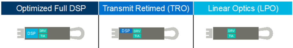
Architecture Comparison:
Traditional Module (Leftmost diagram):
- Contains: DSP + Driver + TIA
- Full signal processing in module
LPO Module:
- DSP removed from module
- DSP functionality moved to switch ASIC
- Retains: Driver + TIA only
Benefits:
- ~25% cost reduction vs. DSP-based transceivers
- ~50% power savings (typical: 8W vs. 12-15W for 400G)
- Reduced latency (no DSP processing delay)
Limitations:
- Requires advanced host ASIC with robust SerDes capability
- Limited reach: Typically 500m maximum for DR applications
- Reduced link margin: Less tolerance for fiber impairments
- Not suitable for long-haul or challenging environments
Market Position:
- Likely transition technology toward CPO
- Gaining traction for intra-DC applications where switch ASICs have advanced equalization (Broadcom Tomahawk 5, NVIDIA Spectrum-4)
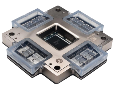
2.7 CPO (Co-Packaged Optics)
Concept: Broadcom’s strength in both ASICs and lasers naturally leads to integration attempts
Architecture: Switch ASIC and optical engine packaged together into single unit
Advantages (Integration Benefits):
- Lower latency
- Lower power consumption
- Higher speeds
Disadvantages:
- Inflexibility (Major Drawback):
- Non-pluggable: Cannot swap modules
- Vendor lock-in: Cannot choose different manufacturers
- Fixed configuration: All ports determined at manufacture
- Traditional: Use some ports now, others later as needed
- CPO: All capabilities fixed, no flexibility
- Physical Limitations:
- ASIC size constraints limit peripheral optical modules
- Typically only 16 optical modules can fit around ASIC
- Physical dimension restriction
- Reliability Concerns:
- Complete package replacement on any failure
- Higher maintenance costs vs. swappable modules
Broadcom’s Projections:
- Claims 80% power reduction – quite significant
- Should capture certain market segments
Market Outlook:
- CPO extremely inflexible compared to pluggable modules
- LPO more likely transition path
- CPO may serve niche applications requiring maximum integration
2.8 Parallel Optics Implementation
Universal Architecture: All optical module structures are inherently parallel:
- Laser arrays
- Photodetector arrays
- Multi-channel fiber (MPO)
- Wavelength division multiplexing
- Multi-channel SerDes on electrical interface
Everything is parallel from end to end
Example: 800G OSFP Module Detailed Breakdown
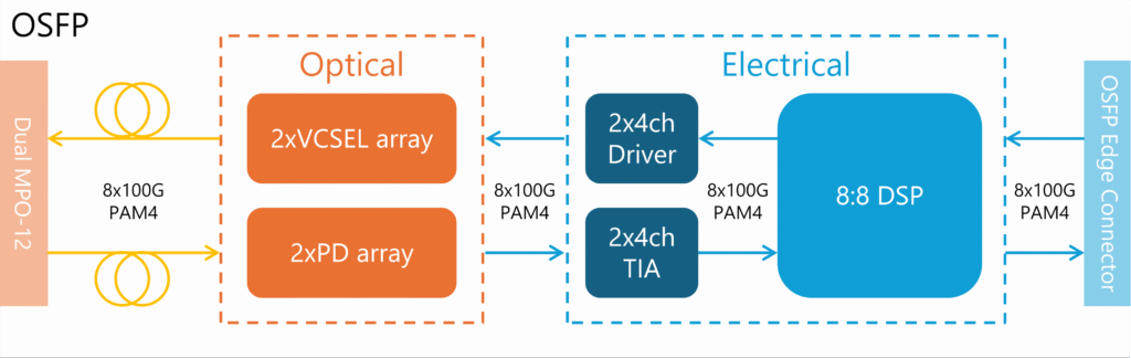
Optical Interface (Dual MPO-12):
- 8 fiber pairs (8 transmit, 8 receive)
Transmit Side:
- Laser: 8-channel VCSEL array (actually 2×4-channel arrays)
- Driver: 8-channel (2×4-channel configuration)
- DSP: Processes 8× 100G signals
Receive Side:
- Detector: 8-channel PIN photodiode array
- TIA: 8-channel (2×4-channel configuration)
- DSP: Processes 8×100G signals
Electrical Interface (Switch side):
- SerDes: Each lane is 100G (NOT 800G)
- Current standard: Actually 112 Gbps per lane
- Note: NOT 800G serialized interface
Future Evolution:
- 1.6T modules: Single channels will upgrade to 200G
- This should become the mainstream approach
Key Insight: We achieve high aggregate speeds entirely through parallel architecture, not higher single-lane speeds
3. Performance Specifications and Metrics
Understanding these metrics helps when customers evaluate optical modules and prevents less scrupulous vendors from exploiting customer knowledge gaps.
Important Note: Different manufacturers may intentionally confuse these specifications when dealing with uninformed customers (e.g., claiming “our BER is 10⁻¹², yours is only 10⁻⁴!”).
Reality Check: Boundary optical modules from major vendors (Broadcom, Marvell chips) assembled by various manufacturers typically show minimal specification differences. The core components are the same.
3.1 End-to-End Link Performance
Pre-FEC vs. Post-FEC Bit Error Rate (BER)
CRITICAL DISTINCTION – Must Separate These:
Pre-FEC BER (Before FEC correction):
- Typical value: ≈10⁻⁴ (PAM4 systems)
- Reflects raw optical link quality
- Measures cumulative impact of noise, dispersion, crosstalk
Post-FEC BER (After FEC correction):
- Strong DSP: Can achieve 10⁻¹⁵
- Weaker DSP: Achieves 10⁻¹²
- Final link reliability measure
- Cost tradeoff: Better FEC = higher power consumption
Warning: Vendors may try to compare their post-FEC BER (10⁻¹²) against your pre-FEC BER (10⁻⁴) to claim superiority. Know the difference!
Power Consumption
Staggering Cumulative Impact Example:
- Single 800G module: 15W
- Full deployment (64 modules): 64 × 15W = 960W
- System total power: ~2,280W
- Optical modules alone: ~45-50% of total system power
Important Calculation Correction:
- Above is one-sided only
- Data transmission requires both sides
- Actual optical module contribution: Must multiply by 2
Power Consumption by Module Type:
| Module Type | Typical Power | Range | Note |
| 100G QSFP28 | 3.5W | 2.5-4.5W | |
| 400G QSFP112 | 6-8W | 5-10W | |
| 400G OSFP | 10-15W | 8-18W | |
| 800G QSFP-DD | 12-15W | 10-18W | |
| 800G OSFP112 | 15-20W | 12-25W |
Latency
Optical Module Latency Contribution (Often Overlooked):
With DSP:
- Module latency: ~100 nanoseconds
- Comparison: Switch latency is ~400-500ns (or slightly more)
- Implication: Module contributes significant portion of total latency
Without DSP (LPO):
- Module latency: 1-5 nanoseconds only
- Benefit: Negligible, can be essentially ignored
- Major advantage of LPO architecture
Components of Module Latency:
- Optical propagation: ~5 ns/m (negligible internally)
- Electro-optic conversion: 1-5 ns
- DSP processing: 100-100 ns (dominant factor)
- Electrical I/O: 1-10 ns
Link Budget
Definition: Ratio of transmitted optical power to received optical power—essentially the maximum allowable optical path loss.
Performance Indicator:
- Larger ratio = Better module performance
- Ability to use less transmit power while achieving better reception quality
Calculation:
Link Budget (dB) = TX Maximum Power (dBm) - RX Sensitivity (dBm)Application: Less commonly referenced but important for understanding module capabilities
Typical Link Budgets:
- SR applications (MMF): 3-7 dB
- DR/FR applications (SMF, 2km): 8-11 dB
- LR applications (SMF, 10km): 12-16 dB
- ER/ZR applications (SMF, 40-80km): 18-28 dB
3.2 Transmitter Specifications
Average Launch Power (Pout)
Unit: dBm (decibel-milliwatts) – logarithmic power measurement
Operating Range: Has both maximum and minimum limits
Why Limits Matter:
- Too high:
- Higher power consumption
- Risk: Can damage/burn the receiver detector
- Too low:
- Increases the bit error rate at the receiver
- Insufficient signal strength
Must operate within reasonable range
Typical Ranges:
- SR (850nm VCSEL): -7 to +2 dBm per lane
- DR (1310nm DFB): -6 to +4 dBm per lane
- FR4 (1310nm CWDM): -5 to +5 dBm per wavelength
- ER4 (1550nm DWDM): -2 to +6 dBm per wavelength
TDECQ (Transmitter Dispersion Eye Closure Quaternary)
What It Measures: Transmit-side eye diagram quality
Key Concept: Represents signal degradation degree during transmission
Remember: Lower TDECQ = Better quality
Specifications by Speed:
- 800G: ≤ 3.0 dB
- 400G: ≤ 3.4 dB
- 100G: ≤ 4.5 dB
Trend: Higher-speed modules require better (lower) TDECQ specifications
Professional Awareness: Even if you can’t completely memorize the specification, you should recognize this term when mentioned
Extinction Ratio (ER / OER)
Definition: Ratio of optical power between high level and low level signals
Unit: dB (decibels)
Signal Representation:
- Traditional: Binary 0 and 1
- PAM4: 0, 1, 2, 3 (four levels)
- Future: 0-6 or 0-8 (even more levels possible)
Performance Indicator: Higher value = Better
- Greater power difference between levels
- Easier signal discrimination
Remember: Represents contrast between signal levels—higher contrast improves receiver’s ability to decode
3.3 Eye Diagram Analysis
Origin: Phenomenon observed during debugging when optical signals are fed into oscilloscope
Visual Appearance: Good signals display an eye-shaped pattern, hence the name
Quality Assessment:
Good Signal (Open Eye):
- Appearance: Resembles well-formed almond-shaped eye
- Characteristics:
- Symmetric shape
- Wide eye opening
- Low jitter
- High signal-to-noise ratio
- Impact: Easy to distinguish 1 and 0 (or multi-level signals)
Poor Signal (Closed Eye):
- Appearance: Poorly formed, narrow opening
- Characteristics:
- Asymmetric
- Narrow eye opening
- High jitter
- Low contrast
- Impact: Difficult to distinguish signal levels, high error rate
Eye Diagram Parameters:
- Eye Height: Amplitude separation between levels
- Eye Width: Timing margin at sampling point
- Eye Opening: Combined metric
- Jitter: Temporal variation
- Noise: Amplitude variation
Practical Advice: Understanding this concept is sufficient—this is quite specialized
TDECQ Connection: TDECQ metric is based on eye diagram measurement, quantifying eye closure degree to measure signal degradation
3.4 Receiver Specifications
Average Receive Power (Pin)
Ideal: Lower is better (can detect weaker signals)
Reality: Too low is also problematic
- Insufficient signal strength
- Increased bit error rate
Balance Required: Must operate within optimal range
Typical Ranges:
- 400G: -6.9 to +4.5 dBm
- 100G: -10.3 to +2.4 dBm
Receiver Sensitivity vs. Average Receive Power
CRITICAL DISTINCTION (Vendors May Confuse These):
Receiver Sensitivity (More Commonly Used):
- Definition: Minimum optical power required to receive signal at a specific BER
- Better metric because it’s defined with BER context
- More practical for real-world applications
Average Receive Power:
- Simple power measurement
- Less meaningful without BER context
Vendor Tactic Warning:
- Some vendors use “Minimum Receive Power” to confuse comparison with “Receiver Sensitivity.”
- These are different metrics!
Values Comparison:
- Receiver Sensitivity: Appears numerically larger (includes BER requirement)
- Minimum Receive Power: Can be lower (no BER consideration)
When comparing: Ensure you’re comparing like metrics, not mixing sensitivity with minimum power
Typical Sensitivity Values:
- 100G PAM4 (PIN): -10 to -12 dBm
- 400G PAM4 (PIN): -8 to -10 dBm
- ER/ZR (APD): -18 to -24 dBm
Damage Threshold (Rdam)
Definition: The maximum optical power receiver can withstand before permanent damage
Purpose: Protective specification
Risk: Exceeding this threshold burns out the photodetector
Implication:
- Stronger transmit power is NOT always better
- Improper tuning can destroy receiver components
- Transmit-receive pairing requires careful calibration
Typical Values: +3 to +5 dBm above maximum receive power specification
4. Network Deployment Scenarios
4.1 Basic Point-to-Point Connectivity
Simple Case: Direct connection between two optical modules
- Straightforward, no special considerations
- Just connect and operate
However, must address the special case of 800G modules…
4.2 Critical 800G Architecture Understanding
Fundamental Principle (Previously Explained):
- Majority of 800G modules = Two 400G modules physically combined
- Integrated into single OSFP form factor
- Two MPO-12 interfaces (separate optical ports)
Direct Connectivity Capability:
- Can connect directly to two separate 400G modules via two fiber cables
- No conversion required
Cross-Form-Factor Compatibility:
Example: One 800G OSFP-VR4 module can directly connect to:
- One 400G OSFP-VR4 module (via one MPO-12 cable)
- One 400G QSFP112-VR4 module (via another MPO-12 cable)

Key Point:
- Electrical connector form (OSFP vs. QSFP) does NOT affect optical interconnection
- Optical signal compatibility is what matters
- Only requires MPO-12 optical cables for connection
- No conversion or adaptation needed
4.3 NVIDIA Reference Architecture
Understanding NVIDIA’s ecosystem helps with project deployments:
Switch Side:
- 800G modules: Called “2-port” or “dual-port”
- Literally two separate ports
- Heat sink: Fin-Top configuration
- Form factor: OSFP
NIC/DPU Side (Two Product Lines):
ConnectX Series:
- Flexible: Supports both OSFP and QSFP112 modules
- Can use either form factor
BlueField DPU Series:
- Restricted: Only supports QSFP112
- Cannot use OSFP modules
Project Implications: When configuring servers with NVIDIA NICs/DPUs, pay attention to form factor compatibility:
- ConnectX: Either OSFP or QSFP112 works
- BlueField: Must specify QSFP112 only
4.4 Breakout Configurations (1:N via Optical Harness)
Terminology: Use “harness” or “breakout cable,” not “optical splitter”
800G Flexibility: Since 800G = 8×100G channels, can break out in multiple ways:
- 1:2 (800G → 2×400G)
- 1:4 (800G → 4×200G)
- 1:8 (800G → 8×100G)
Common Harness Types
| Harness Type | Configuration | Application |
| MPO-16 to Dual MPO-12 | 1×MPO-16 → 2×MPO-12 | 800G SR8 → 2×400G SR4<br>Spine (800G) to legacy leaf (400G) |
| MPO-16 to 8×LC Duplex | 1×MPO-16 → 8×LC pairs | 800G SR8 → 8×100G SR<br>Aggregation to access switches |
| MPO-12 to 4×LC Duplex | 1×MPO-12 → 4×LC pairs | 400G SR4 → 4×100G SR<br>Core to distribution |
| MPO-8 to LC/SC | 1×MPO-8 → Multiple LC/SC | Data center short-reach |
| Dual MPO-12 to 8×LC | 2×MPO-12 → 8×LC pairs | 800G → 8×100G breakout |
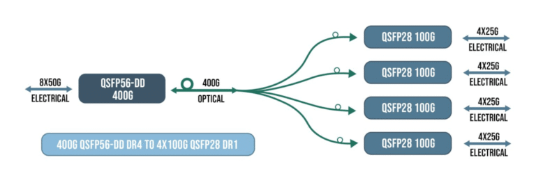
Typical Application: 800G to 8×100G Breakout
Very Common Scenario:
Configuration Details:
- 800G side: DR8 specification
- 100G side: DR1 specification (special format)
- Harness: Two 1:4 breakout cables
- Each converts MPO-12 → 4×LC duplex
- Total: 8×LC duplex connections
Important Note: This specific configuration (DR8↔DR1) is particularly common—be aware of it
Advantages of Harness/Breakout Approach:
- Infrastructure reuse: Leverage existing lower-speed ports
- Migration flexibility: Gradual upgrade paths
- Cost optimization: Deploy higher-speed modules only where needed
- Reduced cabling complexity: Single MPO vs. multiple LC runs
4.5 Intra-Data Center Architecture
Typical Topology: Leaf-Spine architecture
GPU Servers (400G NICs)
    ↓ 800G VR4/SR4 (50-100m)
ToR Switch (Leaf) - CX864E-N
    ↓ 800G SR8/DR8/FR8/LR8 (100m-10km)
Spine Switch - CX864E-N
Module Recommendations:
Server to ToR:
- 800G OSFP-2VR4 (50m, OM4)
- 400G OSFP-VR4 (50m, OM4)
- 400G QSFP112-VR4 (50m, OM4)
ToR to Spine (CX864E-N as ToR):
- 800G OSFP-SR8 (100m, OM4, dual MPO-12)
- 800G OSFP-DR8 (500m, SMF, dual duplex LC)
- 800G OSFP-FR8 (2km, SMF)
- 800G OSFP-LR8 (10km, SMF)
400G Connectivity:
- 400G SmartNIC connections
- 400G DPU connections
4.6 Our Optical Module Portfolio
Complete Range: 1G to 800G comprehensive matrix
Distance Coverage by Speed:
- 800G: VR → SR → DR → FR → LR (complete lineup)
- 400G: Including higher-end ER options
- Lower speeds: Full coverage
Important: 200G Compatibility Issue
The 200G Problem:
Why Awkward:
- Uses 4×56 Gbps lane speed
- Incompatible with both:
- 400G: Uses 4×112 Gbps
- 100G: Uses 4×28 Gbps (or sometimes 112 Gbps)
Practical Impact:
- CX664: Works great in homogeneous 200G networks
- Cross-speed connectivity: Very difficult
- Cannot easily split to 100G
- Cannot easily combine to 400G
- 2:1 or 1:2 conversions problematic
Industry-Wide Issue: 200G is an awkward speed across the entire industry
- Historical artifact of technology evolution
- Doesn’t align well with speeds above or below
- Recommendation: Be aware of this limitation in projects
Cause: During technology evolution, this intermediate speed emerged but now doesn’t mesh well with current mainstream speeds.
4.7 Our Product Naming Convention
Format Structure: OT-[Speed]-[Form Factor]-[Distance Type]
Example 1: OT-400G-QDD-VR4-MPO12
- OT: Optical Transceiver
- 400G: Speed
- QDD: QSFP-DD (electrical interface type)
- VR4: Very Short Range, 4 channels
Detailed Specifications (from example):
- Channel configuration: 8 channels (QSFP-DD = 2×QSFP)
- Per-lane speed: 56 Gbps (8×56 = 400G? Actually 8×50)
- Optical fiber: 850nm multimode fiber
- Maximum distance: 50 meters (OM3/OM4)
- Power consumption: 8W
Our 800G Modules: Key Selling Points
Competitive Advantages:
- Silicon Photonics Technology:
- All our 800G modules use silicon photonics
- Lower power consumption vs. traditional InP lasers
- Industry-Leading Power Efficiency:
- 13.5W typical consumption
- Among the lowest in the industry
- Significant advantage in large deployments
- Customer Value:
- Lower operating costs
- Reduced cooling requirements
- Better suited for high-density deployments
4.8 Lower-Speed Modules (10G-100G)
Portfolio: Comprehensive 10G to 100G offerings
Recommendation: Review specifications as needed for specific projects
- Contact me directly for questions
- Pricing: Competitive across the board
- Quality: Excellent performance
- Integration: Can be easily specified in projects
5. Additional Technical Considerations
5.1 APC vs. UPC Connector Types
Question from Training: What’s the difference between APC and UPC?
Physical Difference:
- Cutting angle of the fiber end-face
- UPC (Ultra Physical Contact): Straight cut (perpendicular)
- APC (Angled Physical Contact): Angled cut (~8 degrees)
Performance Impact:
- APC: Angled cut provides larger contact surface area
- Better fiber-to-fiber alignment
- Lower insertion loss
- Higher return loss (less back-reflection)
Usage Pattern:
- 400G/800G: Predominantly APC connectors
- Our modules: Basically all APC
- Better performance for high-speed applications
Practical Importance: More relevant for after-sales and engineering teams
- Specify correct type when ordering
- Match connector types on both ends
5.2 Optical Signal Compatibility Rules
Fundamental Principle: Two optical modules can interconnect if their optical signal specifications match, regardless of electrical connector differences.
Key Compatibility Factor: Lane speed (baud rate)
Matching Examples:
- 56 Gbps ↔ 56 Gbps: Compatible
- 112 Gbps ↔ 112 Gbps: Compatible
- 28 Gbps ↔ 28 Gbps: Compatible
Incompatible Examples:
- 56 Gbps ↔ 112 Gbps: NOT compatible
- 28 Gbps ↔ 56 Gbps: NOT compatible
5.3 100G Modulation Format Incompatibility
Critical Understanding: Not all 100G modules are compatible with each other
Two Incompatible 100G Formats:
100G DR1 (Single-lane 100G):
- Configuration: 1×100 Gbps
- Modulation: PAM4
- Compatible with: 800G breakout (8×100G DR1)
- Product code: OT-100G-QSFP-DR1
100G SR4 (Four-lane 100G):
- Configuration: 4×25 Gbps
- Modulation: NRZ
- NOT compatible with 800G breakout
- Product code: OT-100G-QSFP28-SR4
- Historical default: When people said “100G QSFP28,” they meant SR4
Why This Matters:
- 800G → 100G breakout: Must use DR1 format
- Legacy 100G: Probably SR4 format
- Cannot mix: DR1 and SR4 are incompatible
Nomenclature Note: There appears to be a typo in documentation—the 100G DR1 should reference 112 Gbps modulation capability.
5.4 BiDi Module Pairing
Special Characteristic: BiDi modules are sold and used in pairs
Configuration:
- Module A (designated “#1”): TX on one wavelength, RX on another
- Module B (designated “#2”): TX and RX wavelengths swapped
Critical: Must use matching pair (#1 with #1’s mate, #2 with #2’s mate)
Single Fiber Application:
- One fiber for TX, one for RX (simplex mode on each fiber)
- Roles reverse on opposite end
Example Pairing:
- 100G SR-BiDi 1.2 ↔ 400G SR4-BiDi 1.2
- Connected via 1:4 breakout
- One transmit, one receive fiber (simplex)
5.5 Heat Sink Type Specification in Product Codes
800G Modules – Three Form Factors:
Switch-Side (Default – No suffix):
- Fin-Top design
- 13mm height
- Higher cooling capacity
- Product code: No “R” suffix
- Example: OT-800G-OSFP-SR8
NIC/Host-Side (With “R” or “RHS” suffix):
- Flat-Top/RHS design
- 8.5mm height
- Lower profile
- Product code: Includes “R“
- Example: OT-800G-OSFP-R-SR8
Critical for Ordering:
- CX864E switch: Order modules without “R” (Fin-Top)
- NVIDIA NICs/DPUs: Order modules with “R” (RHS/Flat-Top)
400G Modules: Same convention applies
- Especially important for NIC-side 400G modules
- All our NIC-side OSFP modules available in “R” versions:
- OT-400G-OSFP112R-SR4
- OT-400G-OSFP112R-DR4
Conclusion
Optical transceivers represent sophisticated optoelectronic systems that justify their premium pricing through:
- Advanced semiconductor integration: Silicon photonics, complex DSPs, precision laser arrays
- Thermal engineering: Active cooling systems consuming power themselves
- Signal processing excellence: 8-10 orders of magnitude BER improvement through FEC
- Manufacturing precision: Submicron alignment tolerances, wavelength stability
Future Directions:
- LPO gaining traction: 50% power savings, cost reduction
- CPO for specific niches: Maximum integration where flexibility isn’t critical
- Silicon photonics expanding: Marvell partnership positions us well
- 1.6T/3.2T emerging: MXC connectors, 200G lanes coming
For any questions not covered in this guide, please reach out directly. Our comprehensive portfolio from 1G to 800G, combined with competitive pricing and silicon photonics technology leadership, positions us excellently for both current projects and future evolution.